经典的转录组差异分析通常会使用到三个工具limma/voom, edgeR和DESeq2。今天我们就通过一个小规模的转录组测序数据来演示DESeq2的简单流程。
文中使用的数据来自Standford 大学的一个拟南芥的small RNA-seq数据(https://bios221.stanford.edu/data/mobData.RData)

该数据包含6个样本:**SL236,SL260,SL237,SL238,SL239,SL240**, 并分成了三组,分别是:
MM="triple mutatnt shoot grafted onto triple mutant root"
WM="wild-type shoot grafted onto triple mutant root"
WW="wild-type shoot grafted onto wild-type root"
简而言之,`WW`组可以认为是实验的对照组,而`MM`和`WM`则是两个处理组。
对于DESeq2的分析流程而言,我们需要输入的数据包括:
- 表达矩阵(
countData)
- 分组信息(
colData)
- 拟合信息(
design):指明如何根据样本的分组进行建模
下面就以mobData 中的数据为例简单介绍DESeq2 的分析流程
载入数据及生成DESeqDataSet
由于mobData 中的行名没有提供基因的ID,我们也不是为了探究生物学问题,就以mobData 的行数作为其ID
cars}1
2
3
4
5
6
7
8
9
10
11
12
13
14
15
16
17
18
19
20
21
22
23
24
25
26
27
28
29
30
31
| library(DESeq2)
library(dplyr)
load("data/mobData.RData")
head(mobData)
## SL236 SL260 SL237 SL238 SL239 SL240
## [1,] 21 52 4 4 86 68
## [2,] 18 21 1 5 1 1
## [3,] 1 2 2 3 0 0
## [4,] 68 87 270 184 396 368
## [5,] 68 87 270 183 396 368
## [6,] 1 0 6 10 6 12
dim(mobData)
## 3000 6
row.names(mobData) <- as.character(c(1:dim(mobData)[1]))
mobGroups <- c("MM", "MM", "WM", "WM", "WW", "WW")
colData <- data.frame(row.names=colnames(mobData),
group_list=mobGroups)
dds <- DESeqDataSetFromMatrix(countData = mobData,
colData = colData,
design = ~group_list,
tidy = F)
dds
## class: DESeqDataSet
## dim: 3000 6
## metadata(1): version
## assays(1): counts
## rownames(3000): 1 2 ... 2999 3000
## rowData names(0):
## colnames(6): SL236 SL260 ... SL239 SL240
## colData names(1): group_list
|
DESeqDataSet 是DESeq2流程中储存read counts和中间统计分析数据的对象,之后的分析都建立在该对象之上进行。
DESeqDataSet 可以通过以下四种方法产生:
- From transcript abundance files and tximport ——
DESeqDataSetFromTximport
- From a count matrix ——
DESeqDataSetFromMatrix
- From htseq-count files ——
DESeqDataSetFromHTseqCount
- From a SummarizedExperiment object ——
DESeqDataSet
预处理
在进行差异分析之前,需要对样本数据的表达矩阵进行预处理,包括:
- 去除低表达量基因
- 探索样本分组信息 – 有助于挖掘潜在的差异样本
1
2
3
4
5
6
7
8
9
10
11
12
13
14
15
16
17
| table(rowSums(counts(dds)==0))
##
## 0 1 2 3 4 5 6
## 1833 442 324 170 92 84 55
keep <- rowSums(counts(dds)==0) < 6
dds.keep <- dds[keep, ]
dim(dds.keep)
## [1] 2945 6
library(factoextra)
library(FactoMineR)
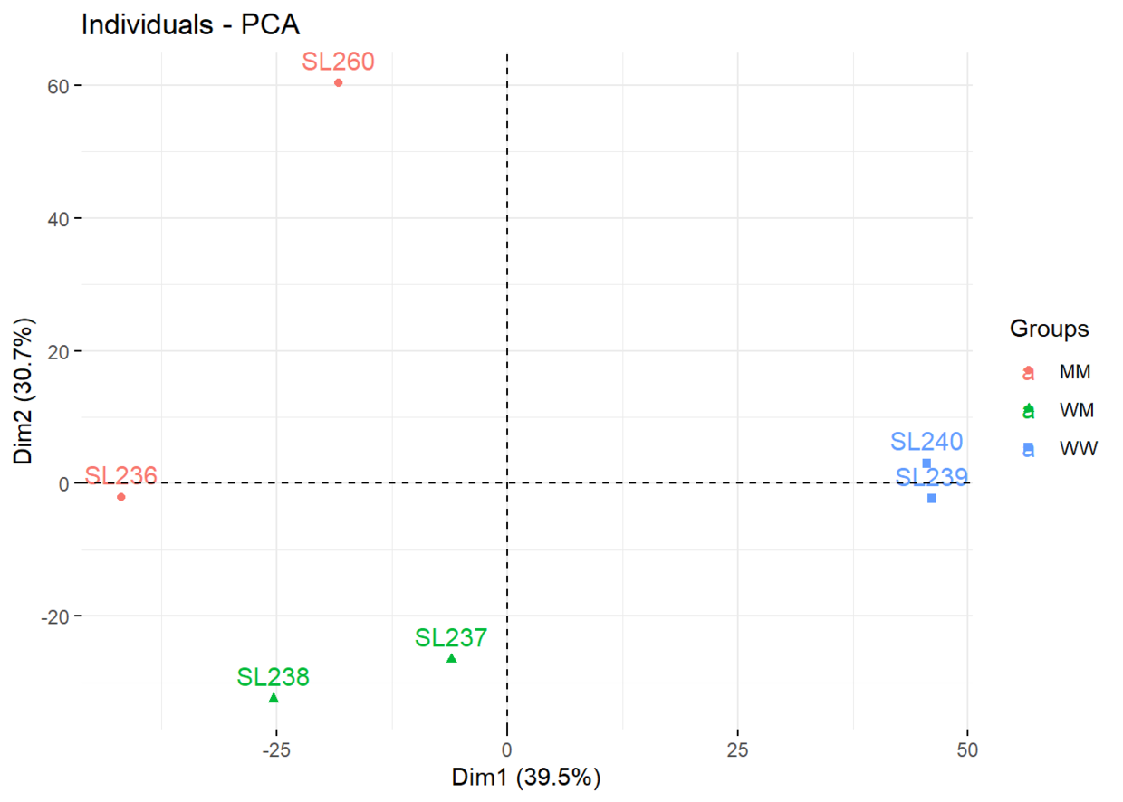
count.pca <- counts(dds.keep) %>% as.matrix %>% t %>% PCA(.,graph = F)
fviz_pca_ind(count.pca,
col.ind = mobGroups,
addEllipses = F,
mean.point = F,
legend.title = "Groups")
|
1
2
3
| colnames(dds.keep) <- c(paste(colnames(dds.keep),mobGroups, sep ="."))
counts(dds.keep) %>% as.matrix %>% t %>% dist %>% hclust %>% plot
colnames(dds.keep) <- colnames(dds)
|
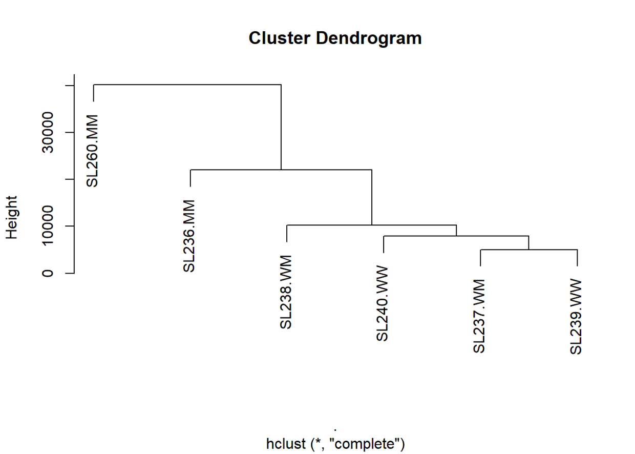
通过PCA结果来看各组样本分组情况还是不错的,但hclust的聚类结果反映的分组就略微有点混杂了,可能要聚类计算的距离函数选用不当有关。
差异分析
使用DESeq()函数进行差异分析时,该函数干了以下三件事:
- 计算文库大小,预测用于标准化的size factor
- 预测离散度(dispersions)
- 使用负二项分布的广义线性回归模型(GLM)进行拟合,以及进行Wald test
The Wald test (also called the Wald Chi-Squared Test) is a way to find out if explanatory variables in a model are significant.
ref : https://www.statisticshowto.com/wald-test/
1
2
3
4
5
6
7
8
9
10
11
| degobj <- DESeq(dds.keep);degobj
## class: DESeqDataSet
## dim: 2945 6
## metadata(1): version
## assays(4): counts mu H cooks
## rownames(2945): 1 2 ... 2999 3000
## rowData names(26): baseMean baseVar ... deviance maxCooks
## colnames(6): SL236 SL260 ... SL239 SL240
## colData names(2): group_list sizeFactor
countdds <- counts(degobj, normalized = T)
deg.res1 <- results(degobj, contrast=c("group_list","MM","WW"), pAdjustMethod = 'fdr')
|
counts() 可以提取DESeq object中的表达矩阵,而results() 可以提取差异分析的结果,其中包括了:
baseMean (样本间的normalized counts均值), log2 fold changes (lfc), lfc standard errors, test statistics, p-values and adjusted p-values.
使用results()函数时需要指明进行比较的样本,这里用 contrast=c("group_list","MM","WW") 提取MM组和WW组进行差异分析的结果。如果想要比较WM组和WW组,只要改变contrast=c("group_list","WM","WW") 即可。
1
2
3
4
5
6
7
8
| # result default
results(object, contrast, name, lfcThreshold = 0,
altHypothesis = c("greaterAbs", "lessAbs", "greater", "less"),
listValues = c(1, -1), cooksCutoff, independentFiltering = TRUE,
alpha = 0.1, filter, theta, pAdjustMethod = "BH", filterFun,
format = c("DataFrame", "GRanges", "GRangesList"), test,
addMLE = FALSE, tidy = FALSE, parallel = FALSE,
BPPARAM = bpparam(), minmu = 0.5)
|
检查结果中是否包含NA值
1
2
3
4
5
6
7
| dim(deg.res1)
## [1] 2945 6
apply(deg.res1,2, function(x) sum(is.na(x)))
## baseMean log2FoldChange lfcSE stat pvalue
## 0 0 0 0 0
## padj
## 1142
|
这里padj中有1142个NA值是因为使用results()提取差异分析结果时,大于alpha值(这里是0.1)的矫正后p-value都会被当做是NA。因此,我们将这些padj值都设为1
1
2
3
4
5
6
7
8
9
10
11
12
13
14
15
16
17
| deg.res1$padj[is.na(deg.res1$padj)] <- 1
table(is.na(deg.res1$padj))
##
## FALSE
## 2945
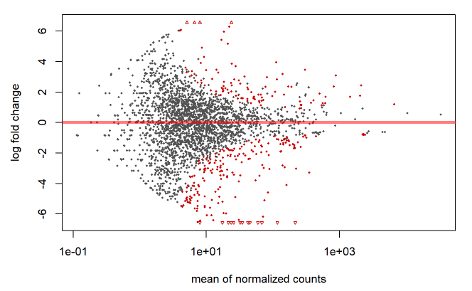
summary(deg.res1)
##
## out of 2945 with nonzero total read count
## adjusted p-value < 0.1
## LFC > 0 (up) : 102, 3.5%
## LFC < 0 (down) : 215, 7.3%
## outliers [1] : 0, 0%
## low counts [2] : 0, 0%
## (mean count < 4)
## [1] see 'cooksCutoff' argument of ?results
## [2] see 'independentFiltering' argument of ?results
plotMA(deg.res1)
|
排序后以log2FoldChange绝对值大于1, padj小于0.05为条件筛选显著的差异表达基因
1
2
3
4
5
6
7
8
9
10
11
12
13
14
15
16
17
18
19
20
21
22
23
24
25
26
27
28
29
30
31
32
| deg.ord1 <- deg.res1[order(deg.res1$padj, decreasing = F),]
deg.sig1 <- subset(deg.ord1,abs(deg.ord1$log2FoldChange)>1 & deg.ord1$padj<0.05)
deg.sig1
## log2 fold change (MLE): group_list MM vs WW
## Wald test p-value: group_list MM vs WW
## DataFrame with 217 rows and 6 columns
## baseMean log2FoldChange lfcSE stat
## <numeric> <numeric> <numeric> <numeric>
## 2500 159.774533763595 -4.11069945121082 0.432943287486228 -9.49477580557611
## 1212 112.711030407211 3.96456274705605 0.449008108800994 8.82960166942819
## 1917 303.58162963147 3.45479344900962 0.406885893259752 8.49081648255649
## 490 71.687159921068 -6.18926587678444 0.753506435554632 -8.21395224345857
## 1317 222.718984861955 -3.03292643435534 0.37190983516799 -8.15500464779421
## ... ... ... ... ...
## 1792 5.98829479907705 -4.93244157414254 1.77616534224116 -2.77701712607386
## 98 6699.69196582045 1.19245883058489 0.429894831042278 2.7738384936934
## 295 6699.58197403621 1.19259109051591 0.429948214187822 2.77380170718637
## 662 5.15806783175131 -5.09298667756621 1.83903942690847 -2.76937329512713
## 899 18.1185589826749 -3.43948745771197 1.24400277511213 -2.76485513257955
## pvalue padj
## <numeric> <numeric>
## 2500 2.20685744092375e-21 3.97896396598552e-18
## 1212 1.05049159823894e-18 9.47018175812401e-16
## 1917 2.05190369014182e-17 1.23319411777524e-14
## 490 2.14024730609951e-16 9.64716473224354e-14
## 1317 3.4916644951535e-16 1.25909421695235e-13
## ... ... ...
## 1792 0.00548602882496584 0.046221074632773
## 98 0.00553991737467495 0.0462481504691228
## 295 0.0055405438166004 0.0462481504691228
## 662 0.00561642447454876 0.0466654992055826
## 899 0.00569480805304419 0.0468846526010898
|
至此,便筛选出了**217个**在`MM`组和`WW`组之间的显著差异表达基因。至于后续的可视化分析则是因课题而异了,等以后有空了再补坑吧!
有同学可能注意到,虽然我们的样本有多个组,但在差异分析时进行的还是pairwise的分析,为什么我们不可以三个组一起分析呢?学过ANOVA的同学应该都知道,ANOVA就是可以应对这种多组差异分析的情况。但要注意的是,ANOVA只可以告诉我们对于某个基因在这三组中是否存在差异,想要找出是哪一组有其他组别有差异还是需要进行pairwise t-test之类的分析。所以,在这里我们两组两组地进行分析正是出于这个考虑,并且有更方便我们解释差异分析的结果,说明在A组基因的表达量相对于B组的是上调还是下调。另外,本文的差异分析还是处于单因子水平(只有一个变量),至于多因子的差异分析以后研究透了再和大家进行分享。
一点想法:
最近想要整理这些转录组常规分析流程,一来是因为之前学习的时候很零碎,想借此机会系统性地整理这方面的知识。另一方面也是因为我感觉平时做湿实验的时候都讲究个protocol,一些基本的实验,像PCR这种我们只要根据具体实验调整一些参数就都可以跟着protocol来做了。所以,一些经典的生信分析也可以有一个这样的“protocol”,要用的时候调整参数就可以了。
Ref:
- https://web.stanford.edu/class/bios221/labs/rnaseq/lab_4_rnaseq.html
- https://www.researchgate.net/post/How_to_interpret_results_of_DESeq2_with_more_than_two_experimental_groups
- https://bioconductor.org/packages/release/bioc/vignettes/DESeq2/inst/doc/DESeq2.html#htseq
- https://bioconductor.org/packages/release/bioc/manuals/DESeq2/man/DESeq2.pdf
完。