Following tutorial from 2019 Nature Protocol (https://www.nature.com/articles/s41596-018-0103-9)
Prerequisite
Project directory: Pathway_Enrichment_Turorial/
下载后解压于Pathway_Enrichment_Tutorial/data/,压缩包内包括以下文件:
- Supplementary_Methods_Supplementary_protocols.pdf
- Supplementary_Table1_Cancer_drivers.txt
- Supplementary_Table2_MesenvsImmuno_RNASeq_ranks.rnk
- Supplementary_Table3_Human_GOBP_AllPathways_no_GO_iea_July_01_2017_symbol.gmt
- Supplementary_Table4_gprofiler_results.txt
- Supplementary_Table5_hsapiens.pathways.NAME.gmt
- Supplementary_Table6_TCGA_OV_RNAseq_expression.txt
- Supplementary_Table7_TCGA_OV_RNAseq_classes.cls
- Supplementary_Table8_gsea_report_for_na_pos.xls
- Supplementary_Table9_gsea_report_for_na_neg.xls
- Supplementary_Table10_TCGA_RNASeq_rawcounts.txt
- Supplementary_Table11_RNASeq_classdefinitions.txt
- Supplementary_Table12_TCGA_Microarray_rmanormalized.txt
- Supplementary_Table13_Microarray_classdefinitions.txt
Software:
- g:Profiler (R client)
- Java Standard Edition (http://www.oracle.com/technetwork/java/javase/downloads/index.html) is required to run GSEA and Cytoscape.
- GSEA (optional)
- The Cytoscape desktop application (http://www.cytoscape.org/download.php)
- Cytoscape plugins:”EnrichmentMap Pipeline Collection” (http://apps.cytoscape.org/apps/enrichmentmappipelinecollection ); 可以在Cytoscape app store中搜到
R | Pathway enrichment analysis
using g:Profiler
这里使用g:Profiler的R包进行富集分析,也可以使用它的网页版(https://biit.cs.ut.ee/gprofiler/gost进行分析
- 首先,使用Supplementary_Table1_Cancer_drivers.txt中的基因列表进行常规的通路富集。
In R
1 | if (!requireNamespace("gprofiler2")) install.packages("gprofiler2") |
这里选择物种为”hsapiens” - Homo sapiens.
exclude_iea: 排除没有经过人工审核的不靠谱GO注释 (less reliable GO annotations, IEAs)
ordered_query: 把输入的基因认为是排序过的基因列表,以一种GSEA的方式进行通路富集
evcodes: 返回输入基因与相应通路产生交集的基因ID
sources: 富集的数据库,这里选择GO的BP项和Reactome的通路。
Available data sources and their abbreviations are:
- Gene Ontology (GO or by branch GO:MF, GO:BP, GO:CC)
- KEGG (KEGG)
- Reactome (REAC): an open-source, open access, manually curated and peer-reviewed pathway database.
- WikiPathways (WP): an open, collaborative platform dedicated to the curation of biological pathways.
- TRANSFAC (TF): is the database of eukaryotic transcription factors, their genomic binding sites and DNA-binding profiles.
- miRTarBase (MIRNA): miRTarBase has accumulated more than three hundred and sixty thousand miRNA-target interactions (MTIs), which are collected by manually surveying pertinent literature after NLP of the text systematically to filter research articles related to functional studies of miRNAs.
- Human Protein Atlas (HPA): including all the human proteins in cells, tissues, and organs using an integration of various omics technologies.
- CORUM (CORUM): provides a resource of manually annotated protein complexes from mammalian organisms.
- Human phenotype ontology (HP): provides a standardized vocabulary of phenotypic abnormalities encountered in human disease.
同时,我们对富集到的通路进行筛选,排除包含过多基因的通路(大于350个),过少基因的通路(小于5个),以及与输入基因交集过小的通路(小于3个)
1 | # filtered by term_size and intersection_size |
理论上,我们应当在进行通路富集之前进行排除,这样才可以通过排除这类通路来通过统计检验的效力(power),但是gprofiler2::gost()并没有提供这样的参数以供我们设定相应的cutoff
富集的结果保存在$table中
1 | # pathway enrichment results table |
##       query significant  p_value term_size query_size intersection_size
## 95  query_1        TRUE 3.82e-13       142         81                15
## 124 query_1        TRUE 6.31e-12       197        120                18
## 125 query_1        TRUE 6.62e-12       230        120                19
##     precision recall    term_id source                        term_name
## 95      0.185 0.1056 GO:0048732  GO:BP                gland development
## 124     0.150 0.0914 GO:0048762  GO:BP mesenchymal cell differentiation
## 125     0.158 0.0826 GO:0060485  GO:BP           mesenchyme development
##     effective_domain_size source_order                parents
## 95                  16592        15077             GO:0048513
## 124                 16592        15103 GO:0030154, GO:0060485
## 125                 16592        17301 GO:0009888, GO:0048513
##                                                                                      evidence_codes
## 95                          ISS,IDA,ISS,ISS,IMP,ISS,TAS,IEP ISS,IGI ISS,IDA,IMP ISS,TAS,ISS,ISS,IDA
## 124         IMP,IMP,IMP ISS,IMP IGI TAS,IMP,ISS,ISS,TAS,ISS,IMP,IMP,ISS,ISS,IMP,IDA ISS,ISS,IMP,IDA
## 125 IMP,IMP,IMP ISS,IMP IGI TAS,IMP,ISS,ISS,ISS,TAS,ISS,IMP,IMP,ISS,ISS,IMP,IDA ISS,IMP ISS,IMP,IDA
##                                                                                                    intersection
## 95                          NF1,GATA3,FBXW7,ARHGAP35,TBX3,CEBPA,AKT1,SOX9,WT1,HGF,ERBB4,ARID5B,ELF3,FGFR2,BRCA2
## 124     PTEN,GATA3,NOTCH1,CTNNB1,TBX3,EPHA3,SOX9,HGF,ERBB4,MTOR,FOXA1,FGFR2,SMAD4,FOXA2,TGFBR2,SMAD2,AXIN2,EZH2
## 125 PTEN,GATA3,NOTCH1,CTNNB1,TBX3,EPHA3,SOX9,WT1,HGF,ERBB4,MTOR,FOXA1,FGFR2,SMAD4,FOXA2,TGFBR2,SMAD2,AXIN2,EZH2
The result
data.framecontains the following columns:
- term_id - unique term identifier (e.g GO:0005005)
- p_values - hypergeometric p-values after correction for multiple testing in the order of input queries
- significant - indicators in the order of input queries for statistically significant results
- term_size - number of genes that are annotated to the term
- query_sizes - number of genes that were included in the query in the order of input queries
- intersection_sizes - the number of genes in the input query that are annotated to the corresponding term in the order of input queries
- source - the abbreviation of the data source for the term (e.g. GO:BP)
- term_name - the short name of the function
- effective_domain_size - the total number of genes “in the universe” used for the hypergeometric test
- source_order - numeric order for the term within its data source (this is important for drawing the results)
- source_order - numeric order for the term within its data source (this is important for drawing the results)
- parents - list of term IDs that are hierarchically directly above the term. For non-hierarchical data sources this points to an artificial root node.
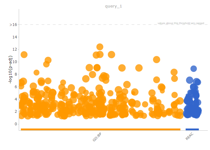
gProfiler2提供Manhattan plot进行通路富集结果的可视化
1 | gostplot(gores1_filtered, capped = TRUE, interactive = TRUE) |
Preparing data for EnrichmentMap
Creating a Generic Enrichment Map (GEM) file
GEM格式文件是Cytoscape EnrichmentMap app中需要的通路富集结果文件。其需要包括GO ID, Description, p-value, FDR, Phenotype and Genes.
由于gost函数输出的p-value已经是多重检验校正后的值,所以这里直接复制两列一样的p-value,其实都是FDR
1 | gem <- gores1_filtered$result[,c("term_id", "term_name", "p_value", "intersection")] |
##          GO.ID                      Description    p.Val      FDR Phenotype
## 95  GO:0048732                gland development 3.82e-13 3.82e-13        +1
## 124 GO:0048762 mesenchymal cell differentiation 6.31e-12 6.31e-12        +1
## 125 GO:0060485           mesenchyme development 6.62e-12 6.62e-12        +1
##                                                                                                           Genes
## 95                          NF1,GATA3,FBXW7,ARHGAP35,TBX3,CEBPA,AKT1,SOX9,WT1,HGF,ERBB4,ARID5B,ELF3,FGFR2,BRCA2
## 124     PTEN,GATA3,NOTCH1,CTNNB1,TBX3,EPHA3,SOX9,HGF,ERBB4,MTOR,FOXA1,FGFR2,SMAD4,FOXA2,TGFBR2,SMAD2,AXIN2,EZH2
## 125 PTEN,GATA3,NOTCH1,CTNNB1,TBX3,EPHA3,SOX9,WT1,HGF,ERBB4,MTOR,FOXA1,FGFR2,SMAD4,FOXA2,TGFBR2,SMAD2,AXIN2,EZH2
保存该文件,在Cytoscape中使用
1 | write.table(gem, file = "extdata/gProfiler_gem.txt", sep = "\t", quote = F, row.names = F) |
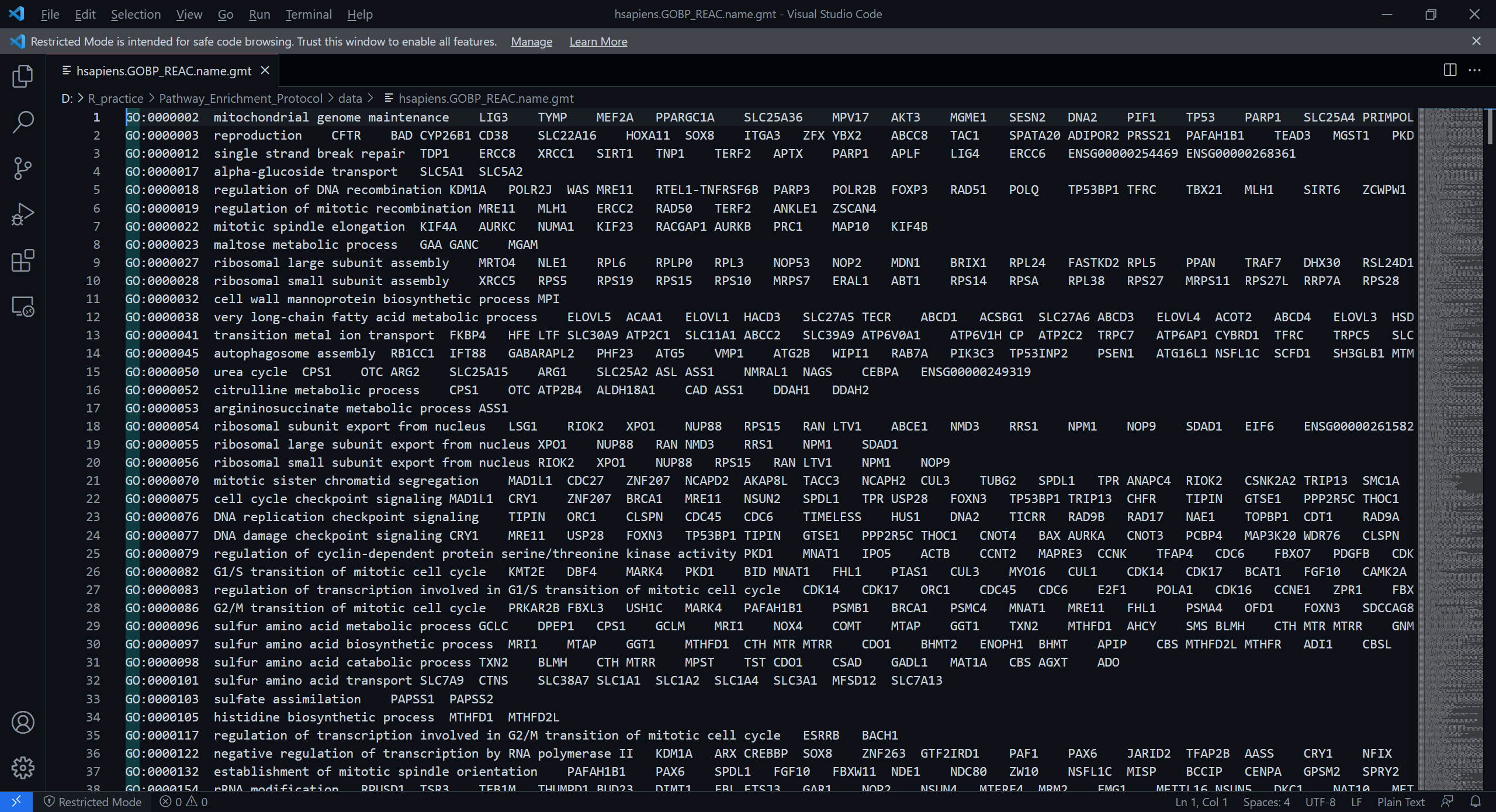
the Gene Matrix Transposed file format (GMT)
GMT格式文件是一种描述基因集的文件格式;其中每一行代表一个基因集 ,GMT示例如下图:
其中第一列为基因集的ID,第二列是基因集的描述,后续的列为该基因集中的基因ID
如果是使用gprofiler进行分析,可以在其网站上下载对应输入基因ID的GMT文件(https://biit.cs.ut.ee/gprofiler/gost)
首先,在Organism的下拉菜单中选择相应物种,我们这里选择Homo sapiens

然后,打开[Data sources]菜单,下载相应基因ID的GMT

我们这里使用symbol作为基因ID,下载name.gmt.zip这个文件
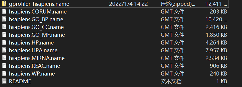
我们这里只使用GO:BP和REAC的注释,故合并这两个文件为hsapiens.GOBP_REAC.name.gmt作为后续分析使用的文件 ,文件的前几行如下所示:
P.S. combined.name.gmt.zip提供的是各个数据库合并后的GMT
另外,gprofiler提供的gmt不包含KEGG和TRANSFAC的数据
“Note that this file does not include annotations from KEGG and Transfac as we are restricted by data source licenses that do not allow us to share these two data sources with our users.”
Cytoscape | Visualization of enrichment results with EnrichmentMap
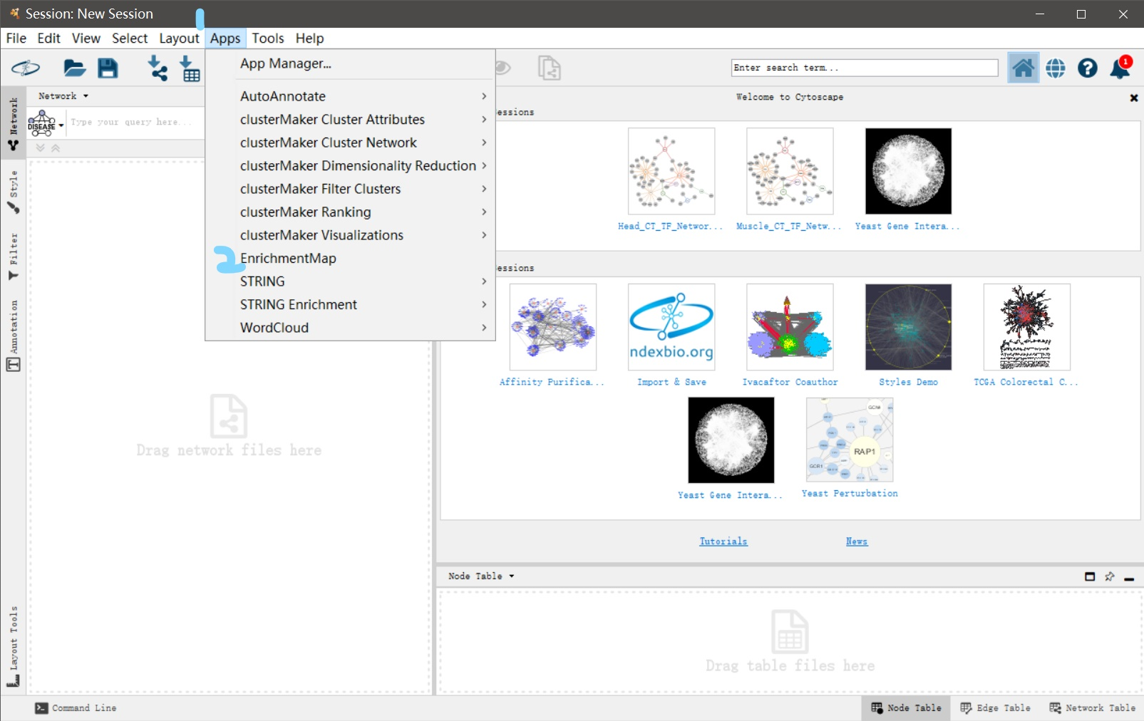
接下来的操作需要在Cytoscape中进行,确保你的电脑安装了Cytoscape,以及其中的EnrichmentMap app
- 打开Cytoscape后,点击上方的[Apps]选项卡
- 打开[EnrichmentMap]
在弹出的Enrichment Map窗口中,
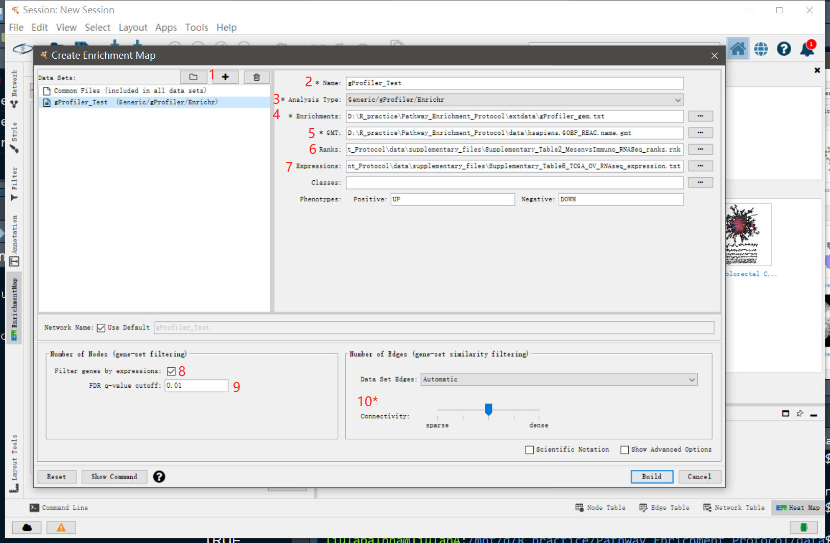
- 点击”+”新建分析
- 修改分析的名字
- 选择富集分析的类型,这里我们选择”Generic/gProfiler/Enrichr”
- 输入GEM格式的富集分析结果,这里输入我们前面保存的
extdata/gProfiler_gem.txt - 输入GMT格式的基因集注释文件,这里输入合并的
hsapiens.GOBP_REAC.name.gmt - (可选)输入基因表达的排序文件,这里我们用文献提供的
Supplementary_Table2_MesenvsImmuno_RNASeq_ranks.rnk - (可选)输入基因表达矩阵文件,这里我们用文献提供的
Supplementary_Table6_TCGA_OV_RNAseq_expression.txt - (可选)根据表达文件进行基因筛选,勾选该选项会对GMT文件的基因进行筛选,排除不在表达文件中的基因。
- (可选)设置每个富集条目的FDR cutoff,高于该cutoff的富集项将会被排除,默认是0.05,这里设置为0.01
- (可选)对网络连接度进行调整。越往左生成的网络越稀疏,越往右生成的网络越密集。本质上是对富集项之间的相关性阈值进行调整,从而减少/增加显示的边。点击[Show advanced options]会显示更多关于网络的调整项目
最后,点击 [Build] 生成网络
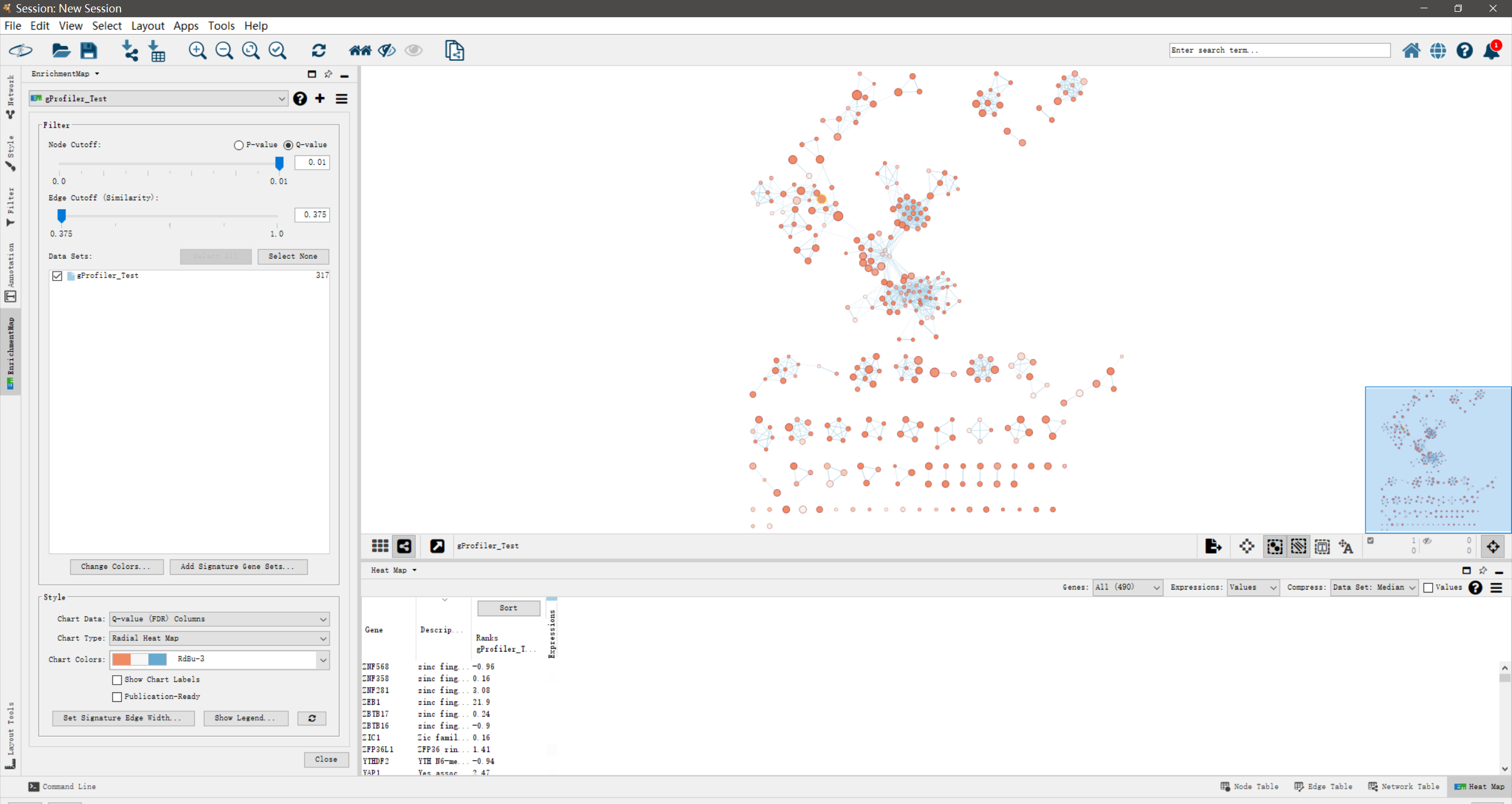
在[Layout]菜单中,可以尝试更换为不同的网络布局,看哪一种布局展示的网络效果最佳,默认为”the unweighted Prefuse Force Directed layout”.
Cytoscape | Auto annotate clustered enriched terms
Enrichment maps typically include clusters of similar pathways representing major biological themes.
富集谱图(Enrichment Map)常常包括了代表主要的生物学主题的
这一节,我们将使用Cytoscape中的”AutoAnnotate” app进行通路clusters的自动注释。
在进行AutoAnnotate前,要确认网络的layout是较优的方案。这是由于它会根据当前的layout进行label。
- 点击[Apps] –> [AutoAnnotate] –> [New Annotation Set…]
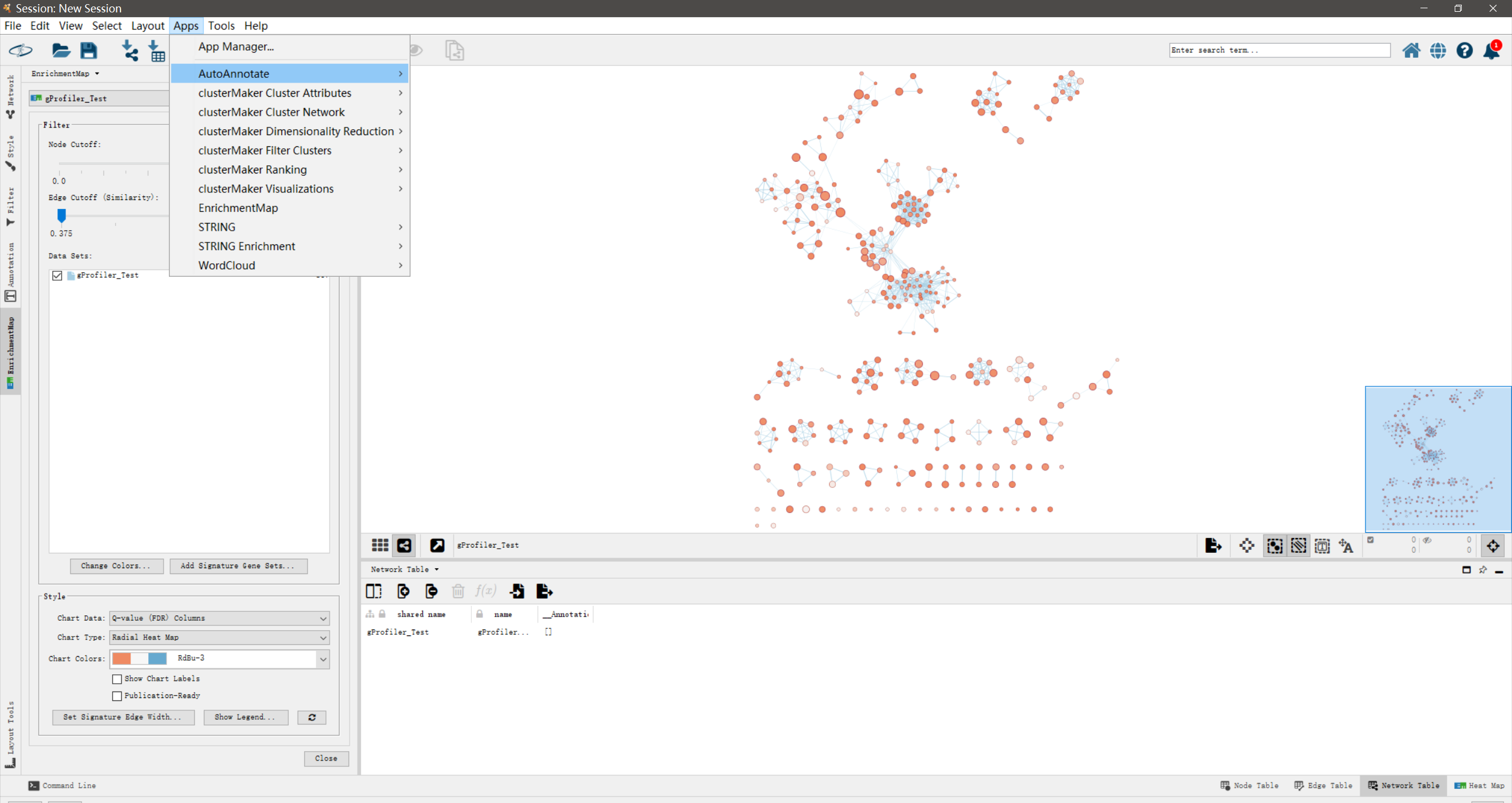
- 在”Quick Start”页面中,点击[Create Annotations]
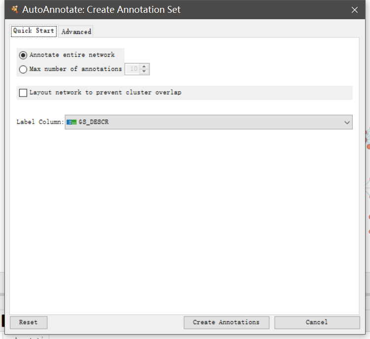
运行后,网络上功能相近的通路节点会被圈为一个cluster,并标注上相应的biological themes。标注的字体越大说明该cluster包含的节点越多。另外,在Control panel中会多了”AutoAnnotations”这一个页面。
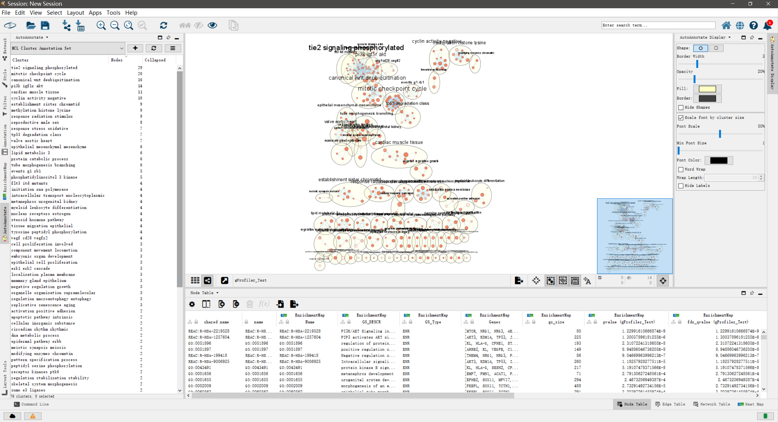
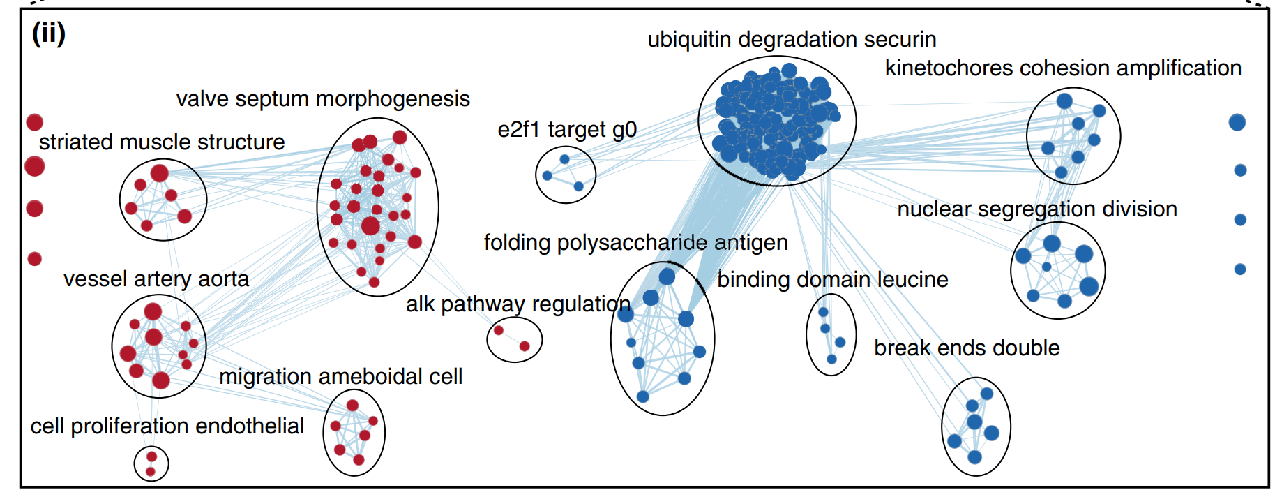
这样生成的注释结果一般是没法看的,我们需要将重叠的圈和标注错开,将”无关的”cluster注释去除,最终达到发表级别的样子
最后,我们可以将运行的cytoscape session保存为.cys文件,方便之后再分析。
在生成富集谱图(Enrichment Map)后更为关键的是对网络的解读!
通路信息天然的具有冗余的特质,因此通路富集分析往往会给出对同一个通路不同描述的注释结果。富集谱图 (Enrichment Map) 简化了冗余的通路信息,将其展示为有代表性的生物学主题 (biological themes),更有利于我们对基因通路富集结果的解读。但这只是相当于帮助我们凝练了通路富集的信息,而对于信息的解读还是依赖于我们的生物学知识。我们需要依据实验的假设、课题的背景做出合理的解释。例如在我们这篇文章的例子中对癌症常见的驱动突变基因进行分析,就发现了许多与肿瘤生长相关的通路。当全面展现出基因集的通路信息后,我们还可以根据感兴趣的通路来寻找相关的基因进行后续分析。总而言之,进行数据分析更为关键的是对数据结果的解读。
Ref
2019 Nature Protocol: https://doi.org/10.1038/s41596-018-0103-9
gprofiler2 vignettes: https://cran.r-project.org/web/packages/gprofiler2/vignettes/gprofiler2.html
Cytoscape: https://cytoscape.org/