使用R建模并预测
1 | library(tidyverse) |
Linear Regression
Model
我们先建一个简单的线性回归模型
1 | model <- lm(dist~speed, cars) |
该模型为: dist = -17.579 + 3.932*speed.
Prediction
Confidence interval
使用 predict 函数根据新的数据进行预测,并给出预测值和其平均值的95%置信区间
1 | speeds <- data.frame(speed=c(10, 20, 53)) |
Prediction interval
给出输入的对应预测值的95%置信区间
1 | predict(model, newdata = speeds, interval = "prediction") |
可视化预测的结果
1 | # 1. Add predictions |
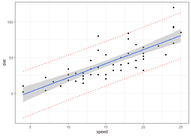
其中,
蓝色的是线性回归拟合曲线
灰色的带为置信区间
红色的虚线为预测值区间
GLM
在R中,广义线性回归使用 glm 函数实现
Model
family 参数选择拟合的回归模型
1 | glm.model <- glm(dist~speed, data = cars, family = gaussian) |
该模型为: dist = -17.579 + 3.934*speed.
与简单线性回归相差不大
Prediction
对于glm对象的prediction,可以设置 se.fit = TRUE
来显示预测的标准误和用于计算标准误的残差
1 | predict(glm.model, newdata = speeds, se.fit = TRUE) |
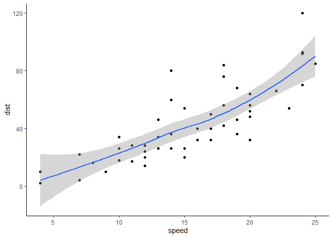
LOESS regression
还可以使用 LOESS (Local Polynomial Regression Fitting) 的方法拟合并预测
1 | cars %>% |
Fitting only
在默认设置下loess拟合模型只能预测处于原始数据range中的值,超出range的值无法预测
1 | cars.lo <- loess(dist~speed, cars) |
Extrapolation
如果想使用loess预测超出range的值,可以设置control = loess.control(surface = "direct")
1 | cars.lo2 <- loess(dist ~ speed, cars, |
但这里需要考虑loess smoothing的span, 如果这个值过小,会过于拟合原始数据,导致预测准确度不高。
以上就是对R中几种线性回归模型建模和预测方法的简述。
完。
ref