scanpy | Preprocessing and clustering 3k PBMCs
本文记录使用scanpy处理3k PBMCs scRNA-seq数据的流程。
环境配置
创建一个虚拟环境以方便管理相关的库。
1 | conda create --name pysc python=3.9 |
本文使用PBMCs 3k数据可以在该网址下载(http://cf.10xgenomics.com/samples/cell-exp/1.1.0/pbmc3k/pbmc3k_filtered_gene_bc_matrices.tar.gz).
下载后,将文件解压至当前的data目录下.
1 | # !mkdir data |
1 | import numpy as np |
1 | sc.settings.verbosity = 3 # verbosity: errors (0), warnings (1), info (2), hints (3) |
e:\miniconda3\envs\pysc\lib\site-packages\umap\distances.py:1063: NumbaDeprecationWarning: [1mThe 'nopython' keyword argument was not supplied to the 'numba.jit' decorator. The implicit default value for this argument is currently False, but it will be changed to True in Numba 0.59.0. See https://numba.readthedocs.io/en/stable/reference/deprecation.html#deprecation-of-object-mode-fall-back-behaviour-when-using-jit for details.[0m
@numba.jit()
e:\miniconda3\envs\pysc\lib\site-packages\umap\distances.py:1071: NumbaDeprecationWarning: [1mThe 'nopython' keyword argument was not supplied to the 'numba.jit' decorator. The implicit default value for this argument is currently False, but it will be changed to True in Numba 0.59.0. See https://numba.readthedocs.io/en/stable/reference/deprecation.html#deprecation-of-object-mode-fall-back-behaviour-when-using-jit for details.[0m
@numba.jit()
e:\miniconda3\envs\pysc\lib\site-packages\umap\distances.py:1086: NumbaDeprecationWarning: [1mThe 'nopython' keyword argument was not supplied to the 'numba.jit' decorator. The implicit default value for this argument is currently False, but it will be changed to True in Numba 0.59.0. See https://numba.readthedocs.io/en/stable/reference/deprecation.html#deprecation-of-object-mode-fall-back-behaviour-when-using-jit for details.[0m
@numba.jit()
e:\miniconda3\envs\pysc\lib\site-packages\tqdm\auto.py:21: TqdmWarning: IProgress not found. Please update jupyter and ipywidgets. See https://ipywidgets.readthedocs.io/en/stable/user_install.html
from .autonotebook import tqdm as notebook_tqdm
scanpy==1.9.3 anndata==0.9.1 umap==0.5.3 numpy==1.24.4 scipy==1.11.1 pandas==2.0.3 scikit-learn==1.3.0 statsmodels==0.14.0 python-igraph==0.10.6 pynndescent==0.5.10
e:\miniconda3\envs\pysc\lib\site-packages\umap\umap_.py:660: NumbaDeprecationWarning: [1mThe 'nopython' keyword argument was not supplied to the 'numba.jit' decorator. The implicit default value for this argument is currently False, but it will be changed to True in Numba 0.59.0. See https://numba.readthedocs.io/en/stable/reference/deprecation.html#deprecation-of-object-mode-fall-back-behaviour-when-using-jit for details.[0m
@numba.jit()
1 | results_file='output/pbmc3k.h5ad' # the file that will store the analysis results |
1 | adata = sc.read_10x_mtx('data/filtered_gene_bc_matrices/hg19/', # the directory with the `.mtx` file |
... reading from cache file cache\data-filtered_gene_bc_matrices-hg19-matrix.h5ad
1 | # remove duplicated symbols |
AnnData object with n_obs × n_vars = 2700 × 32738
    var: 'gene_ids'
我们读入的数据为AnnData格式。
AnnData是python中处理带注释的数据的一种格式,读入的数据并不直接读入内存当中,而是创建与磁盘数据的链接来进行处理。对于单细胞测序数据而言,一般与细胞相关数据存储于.obs,而与feature相关数据存储于.var中

Preprocessing
scanpy包提供的api有几个主要的modules,包括:
- preprocessing:
scanpy.pp, such aspp.calculate_qc_metrics,pp.filter_cells,pp.filter_genes, …; - tools:
scanpy.tl, such astl.pca,tl.tsne,tl.umap, …; - plots:
scanpy.pl, such aspl.scatter,pl.highest_expr_genes,pl.umap, …
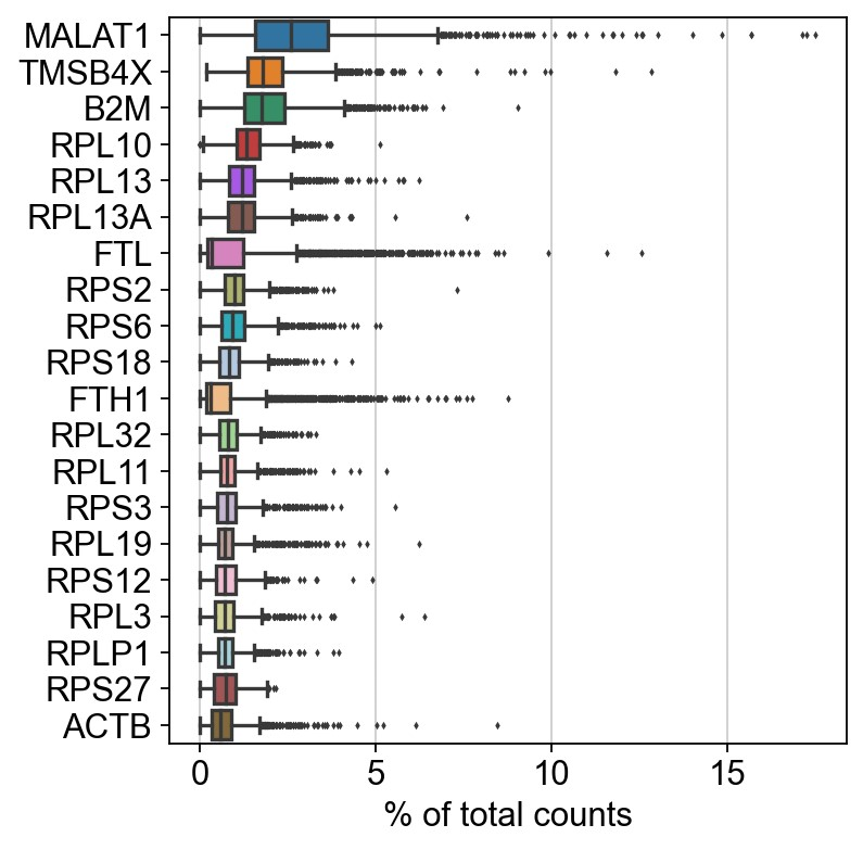
接下来,我们先使用scanpy包进行数据预处理,展示高表达基因在各个细胞中的counts。
1 | sc.pl.highest_expr_genes(adata, n_top=20) |
normalizing counts per cell
    finished (0:00:00)
执行简单的过滤操作。保留至少有200个基因表达的细胞,至少有3个细胞表达的基因。
1 | sc.pp.filter_cells(adata, min_genes=200) |
filtered out 19024 genes that are detected in less than 3 cells
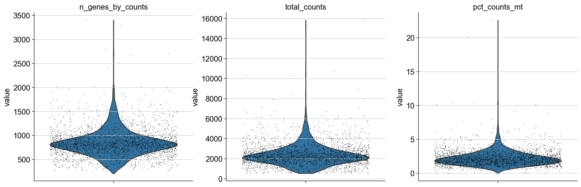
然后,再根据基因的counts和线粒体基因表达进行进一步过滤。
首先,计算线粒体基因比例.
adata.var 存的是feature-level相关的信息,adata.obs 存的是cell-level的信息
1 | adata.var['mt'] = adata.var_names.str.startswith("MT-") |
AAACATACAACCAC-1    3.017776
AAACATTGAGCTAC-1    3.793596
AAACATTGATCAGC-1    0.889736
AAACCGTGCTTCCG-1    1.743085
AAACCGTGTATGCG-1    1.224490
                      ...
TTTCGAACTCTCAT-1    2.110436
TTTCTACTGAGGCA-1    0.929422
TTTCTACTTCCTCG-1    2.197150
TTTGCATGAGAGGC-1    2.054795
TTTGCATGCCTCAC-1    0.806452
Name: pct_counts_mt, Length: 2700, dtype: float32
1 | sc.pl.violin(adata, ['n_genes_by_counts', 'total_counts', 'pct_counts_mt'], jitter=0.4, multi_panel=True) |
e:\miniconda3\envs\pysc\lib\site-packages\seaborn\axisgrid.py:118: UserWarning: The figure layout has changed to tight
  self._figure.tight_layout(*args, **kwargs)
1 | sc.pl.scatter(adata, x='total_counts', y='pct_counts_mt') |
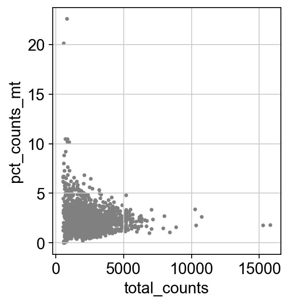
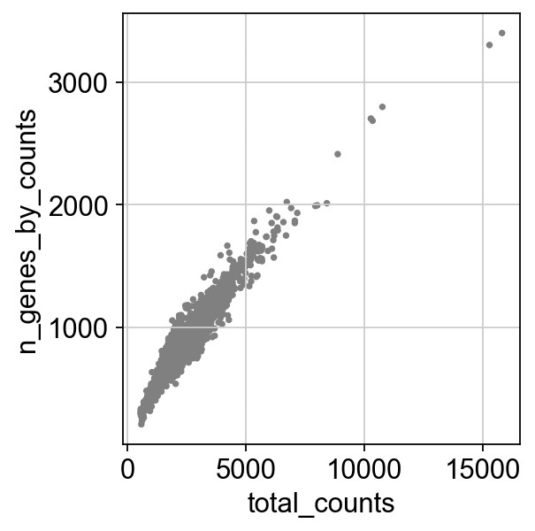
过滤基因数和线粒体基因占比过高的细胞
通过切片的方法过滤
1 | adata = adata[adata.obs.n_genes_by_counts < 2500, :] |
View of AnnData object with n_obs × n_vars = 2638 × 13714
    obs: 'n_genes', 'n_genes_by_counts', 'total_counts', 'total_counts_mt', 'pct_counts_mt'
    var: 'gene_ids', 'n_cells', 'mt', 'n_cells_by_counts', 'mean_counts', 'pct_dropout_by_counts', 'total_counts'
接下来,我们对read counts进行文库大小校正,并进行log转换。
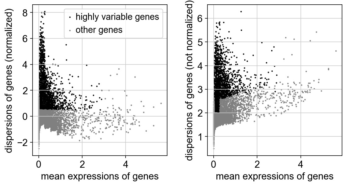
随后,根据normalized expression鉴定highly-variable genes以供后续PCA等分析使用。
1 | # make a copy of raw count |
normalizing counts per cell
    finished (0:00:00)


e:\miniconda3\envs\pysc\lib\site-packages\scanpy\preprocessing\_normalization.py:170: UserWarning: Received a view of an AnnData. Making a copy.
  view_to_actual(adata)
1 | # Identify highly-variable genes |
extracting highly variable genes
    finished (0:00:00)
--> added
    'highly_variable', boolean vector (adata.var)
    'means', float vector (adata.var)
    'dispersions', float vector (adata.var)
    'dispersions_norm', float vector (adata.var)
鉴定的基因存储在adata.var.highly_variable中,后续可被PCA、clustering和UMAP/tSNE等函数识别,所以不需要再对数据进行过滤。
1 | adata.var.highly_variable |
AL627309.1       False
AP006222.2       False
RP11-206L10.2    False
RP11-206L10.9    False
LINC00115        False
                 ...
AC145212.1       False
AL592183.1       False
AL354822.1       False
PNRC2-1          False
SRSF10-1         False
Name: highly_variable, Length: 13714, dtype: bool
这里将adata.raw设置为校正后的数据,以供后续差异分析和可视化使用。相当于是把默认的表达矩阵替换为校正过的。可以通过.raw.to_adata()再替换为原始数据。
1 | adata.raw = adata |
Raw AnnData with n_obs × n_vars = 2638 × 13714
    var: 'gene_ids', 'n_cells', 'mt', 'n_cells_by_counts', 'mean_counts', 'pct_dropout_by_counts', 'total_counts', 'highly_variable', 'means', 'dispersions', 'dispersions_norm'
1 | # filtering hvg |
regressing out ['total_counts', 'pct_counts_mt']
    sparse input is densified and may lead to high memory use
    finished (0:00:03)
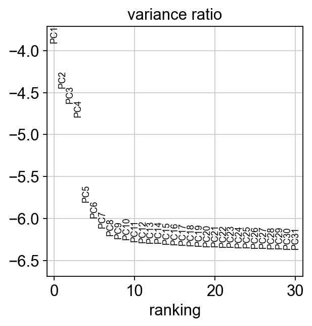
1 | # PCA |
computing PCA
    on highly variable genes
    with n_comps=50
    finished (0:00:00)
1 | adata |
AnnData object with n_obs × n_vars = 2638 × 1838
    obs: 'n_genes', 'n_genes_by_counts', 'total_counts', 'total_counts_mt', 'pct_counts_mt'
    var: 'gene_ids', 'n_cells', 'mt', 'n_cells_by_counts', 'mean_counts', 'pct_dropout_by_counts', 'total_counts', 'highly_variable', 'means', 'dispersions', 'dispersions_norm', 'mean', 'std'
    uns: 'log1p', 'hvg', 'pca'
    obsm: 'X_pca'
    varm: 'PCs'
Computing the neighborhood graph
接下来,我们基于PCA计算细胞的邻接图
1 | sc.pp.neighbors(adata, n_neighbors=10, n_pcs=40) |
computing neighbors
    using 'X_pca' with n_pcs = 40
    finished: added to `.uns['neighbors']`
    `.obsp['distances']`, distances for each pair of neighbors
    `.obsp['connectivities']`, weighted adjacency matrix (0:00:02)
Embedding the neighborhood graph
使用UMAP可视化
1 | sc.tl.umap(adata) |
computing UMAP
    finished: added
    'X_umap', UMAP coordinates (adata.obsm) (0:00:03)
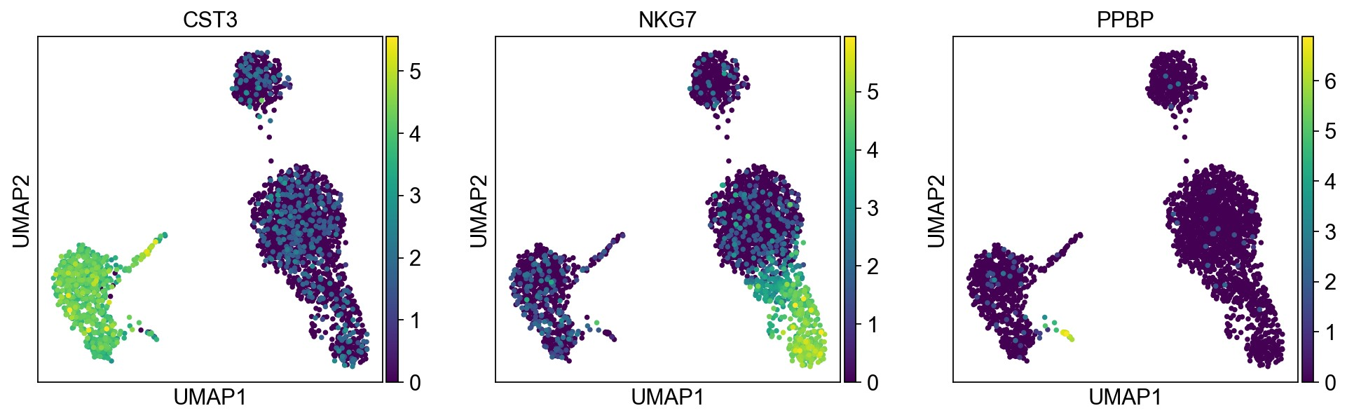
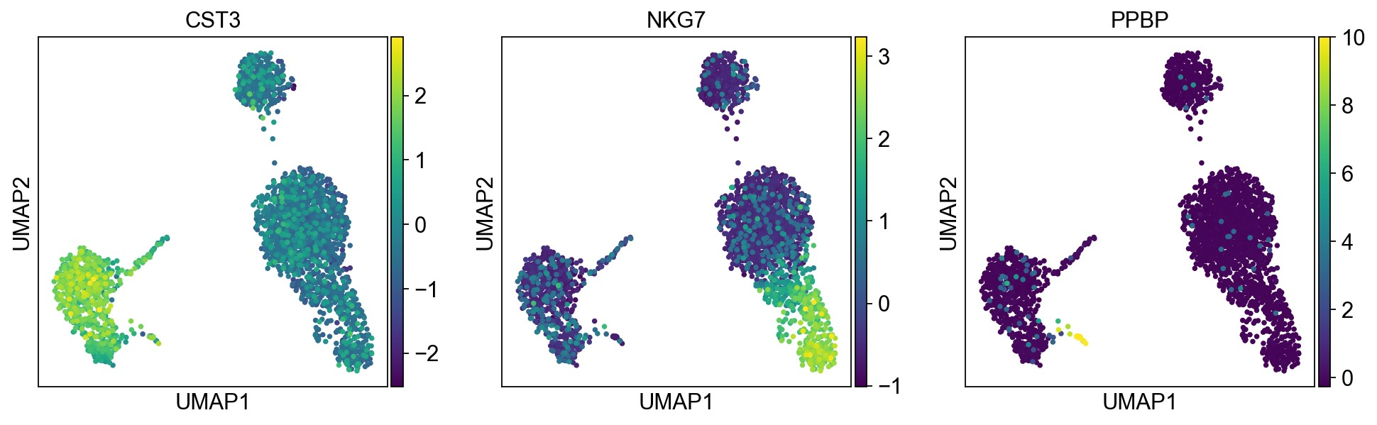
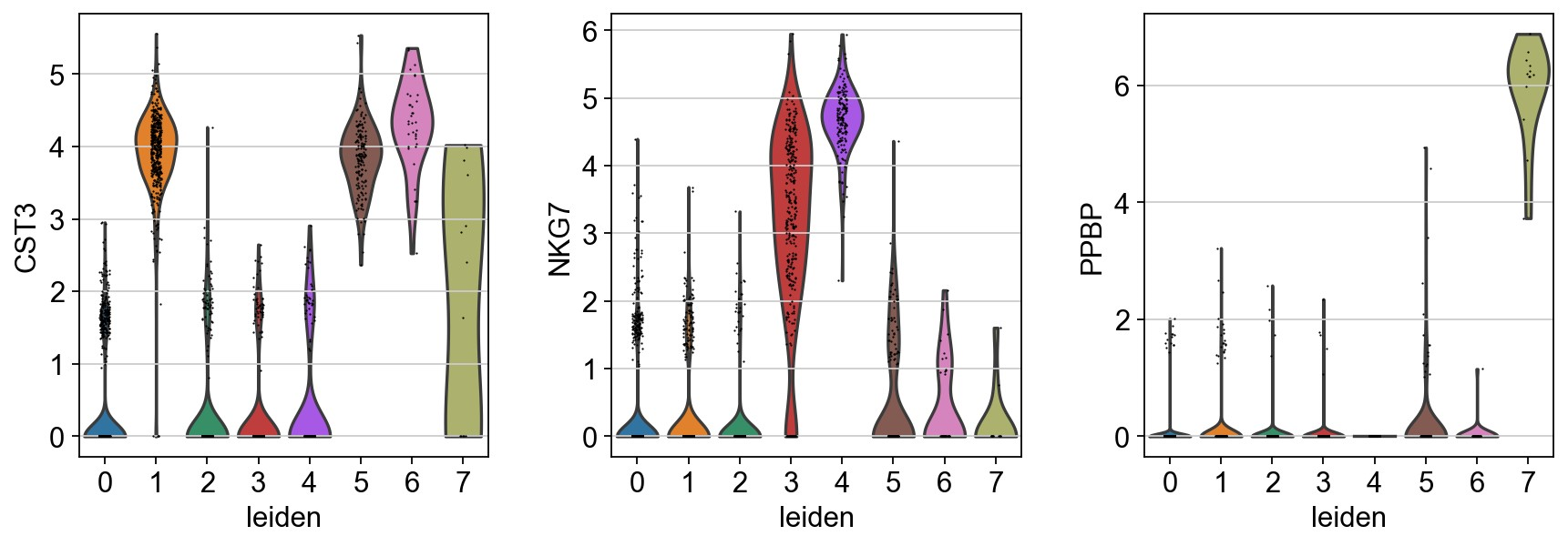
pl.umap默认使用adata.raw中的值作图,由于上面我们将其替换为了normalized后的值。如果想用scaled values作图,可以使用参数use_raw=False
1 | sc.pl.umap(adata, color=['CST3','NKG7', 'PPBP'], use_raw=False) |
Clustering the neighborhood graph
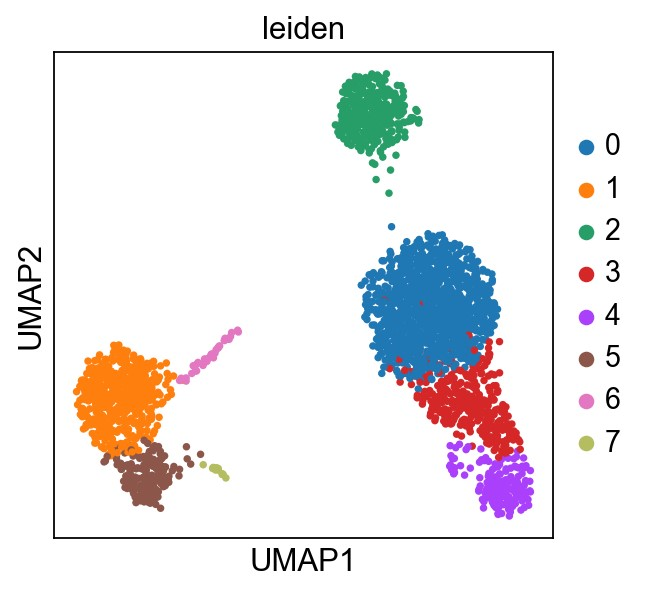
使用Leiden graph-clustering进行聚类
1 | sc.tl.leiden(adata, resolution=1) |
running Leiden clustering
    finished: found 8 clusters and added
    'leiden', the cluster labels (adata.obs, categorical) (0:00:00)


e:\miniconda3\envs\pysc\lib\site-packages\scanpy\plotting\_tools\scatterplots.py:392: UserWarning: No data for colormapping provided via 'c'. Parameters 'cmap' will be ignored
  cax = scatter(
1 | # save the result |
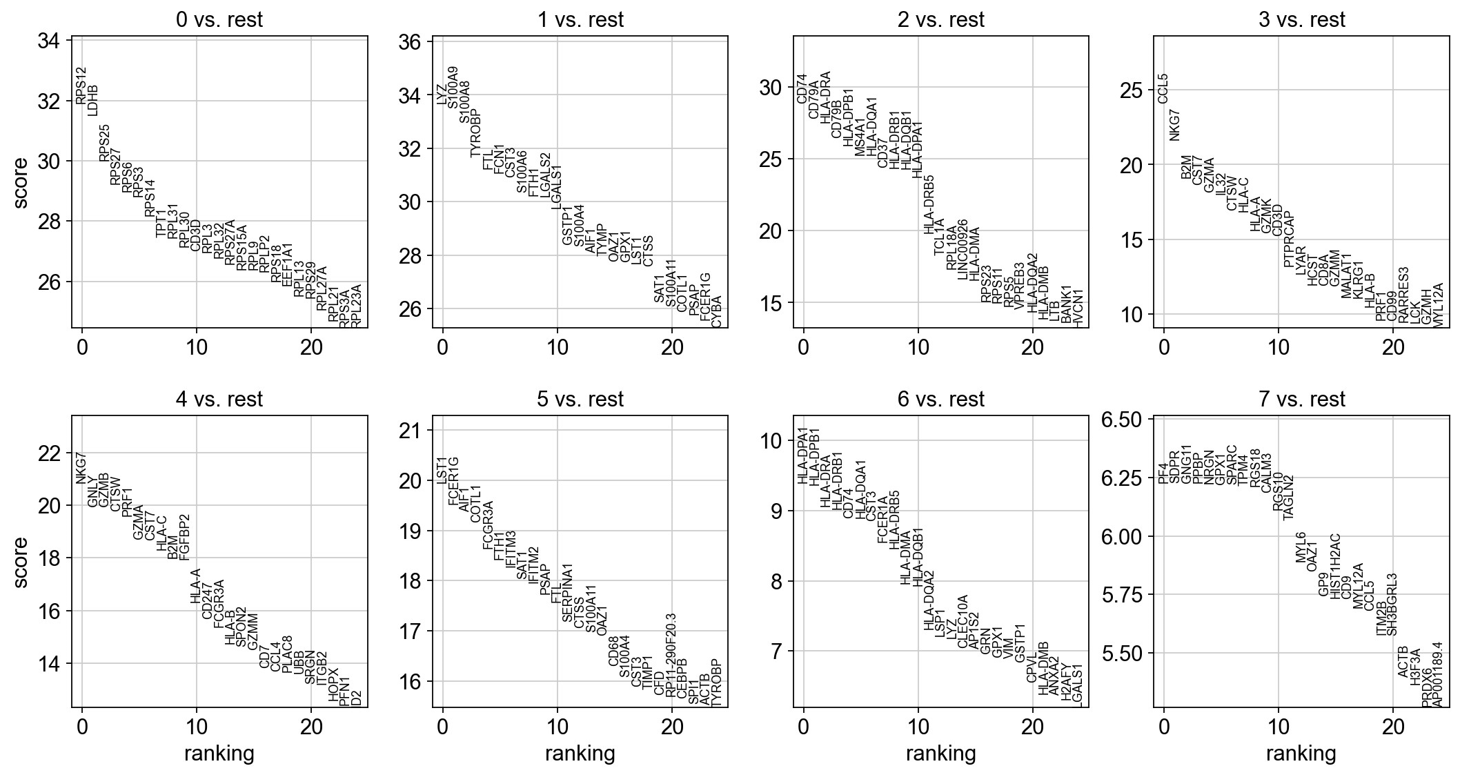
Finding marker genes
Wilcoxon rank-sum test to identify markers
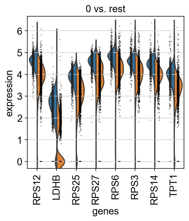
1 | # compare each group with the rest of cell |
ranking genes
    finished: added to `.uns['rank_genes_groups']`
    'names', sorted np.recarray to be indexed by group ids
    'scores', sorted np.recarray to be indexed by group ids
    'logfoldchanges', sorted np.recarray to be indexed by group ids
    'pvals', sorted np.recarray to be indexed by group ids
    'pvals_adj', sorted np.recarray to be indexed by group ids (0:00:01)
1 | adata.write(results_file) |
1 | # marker gene |
| 0 | 1 | 2 | 3 | 4 | 5 | 6 | 7 | |
|---|---|---|---|---|---|---|---|---|
| 0 | RPS12 | LYZ | CD74 | CCL5 | NKG7 | LST1 | HLA-DPA1 | PF4 |
| 1 | LDHB | S100A9 | CD79A | NKG7 | GNLY | FCER1G | HLA-DPB1 | SDPR |
| 2 | RPS25 | S100A8 | HLA-DRA | B2M | GZMB | AIF1 | HLA-DRA | GNG11 |
| 3 | RPS27 | TYROBP | CD79B | CST7 | CTSW | COTL1 | HLA-DRB1 | PPBP |
| 4 | RPS6 | FTL | HLA-DPB1 | GZMA | PRF1 | FCGR3A | CD74 | NRGN |
1 | result = adata.uns['rank_genes_groups'] |
| 0_n | 0_p | 1_n | 1_p | 2_n | 2_p | 3_n | 3_p | 4_n | 4_p | 5_n | 5_p | 6_n | 6_p | 7_n | 7_p | |
|---|---|---|---|---|---|---|---|---|---|---|---|---|---|---|---|---|
| 0 | RPS12 | 1.659522e-223 | LYZ | 7.634876e-249 | CD74 | 2.487145e-183 | CCL5 | 1.674383e-128 | NKG7 | 1.203971e-96 | LST1 | 1.322111e-88 | HLA-DPA1 | 5.422417e-21 | PF4 | 4.722886e-10 |
| 1 | LDHB | 3.010889e-218 | S100A9 | 4.626358e-246 | CD79A | 1.679730e-170 | NKG7 | 5.307754e-104 | GNLY | 1.257170e-88 | FCER1G | 6.259712e-85 | HLA-DPB1 | 7.591860e-21 | SDPR | 4.733899e-10 |
| 2 | RPS25 | 9.032935e-198 | S100A8 | 1.622835e-238 | HLA-DRA | 6.949695e-167 | B2M | 1.364508e-81 | GZMB | 1.429027e-88 | AIF1 | 1.348814e-83 | HLA-DRA | 1.306768e-19 | GNG11 | 4.733899e-10 |
| 3 | RPS27 | 8.254312e-188 | TYROBP | 2.957652e-220 | CD79B | 2.569135e-154 | CST7 | 7.977466e-78 | CTSW | 4.144726e-87 | COTL1 | 5.974694e-82 | HLA-DRB1 | 1.865104e-19 | PPBP | 4.744938e-10 |
| 4 | RPS6 | 8.002057e-185 | FTL | 2.479195e-214 | HLA-DPB1 | 3.580735e-148 | GZMA | 7.266551e-74 | PRF1 | 1.692100e-85 | FCGR3A | 1.392377e-77 | CD74 | 5.853161e-19 | NRGN | 4.800511e-10 |
1 | # compare between groups |
ranking genes
    finished: added to `.uns['rank_genes_groups']`
    'names', sorted np.recarray to be indexed by group ids
    'scores', sorted np.recarray to be indexed by group ids
    'logfoldchanges', sorted np.recarray to be indexed by group ids
    'pvals', sorted np.recarray to be indexed by group ids
    'pvals_adj', sorted np.recarray to be indexed by group ids (0:00:00)
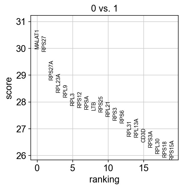
1 | # 0 vs. 1 |
e:\miniconda3\envs\pysc\lib\site-packages\seaborn\categorical.py:166: FutureWarning: Setting a gradient palette using color= is deprecated and will be removed in version 0.13. Set `palette='dark:black'` for same effect.
  warnings.warn(msg, FutureWarning)
1 | # Reload the object with the computed differential expression (i.e. DE via a comparison with the rest of the groups): |
e:\miniconda3\envs\pysc\lib\site-packages\seaborn\categorical.py:166: FutureWarning: Setting a gradient palette using color= is deprecated and will be removed in version 0.13. Set `palette='dark:black'` for same effect.
  warnings.warn(msg, FutureWarning)
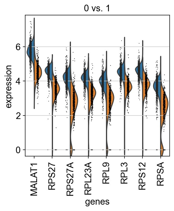
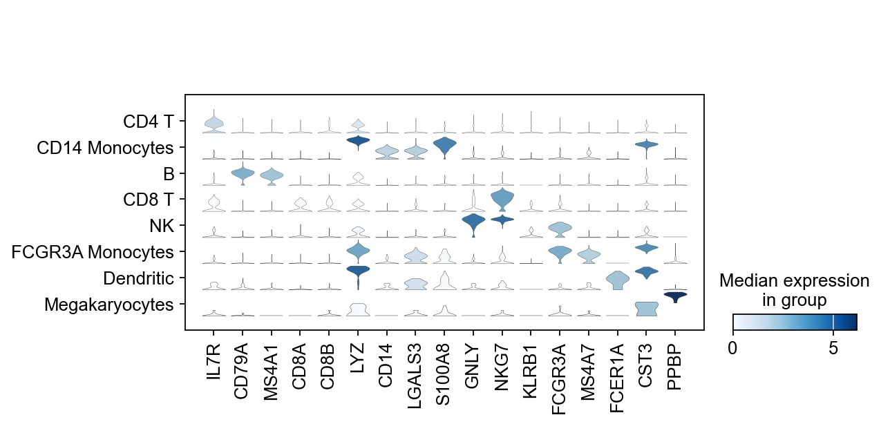
1 | # plot expression across clusters |
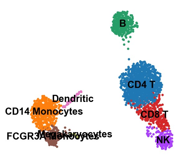
1 | # rename cluster based on cell types |
WARNING: saving figure to file figures\umap.pdf


e:\miniconda3\envs\pysc\lib\site-packages\scanpy\plotting\_tools\scatterplots.py:392: UserWarning: No data for colormapping provided via 'c'. Parameters 'cmap' will be ignored
  cax = scatter(
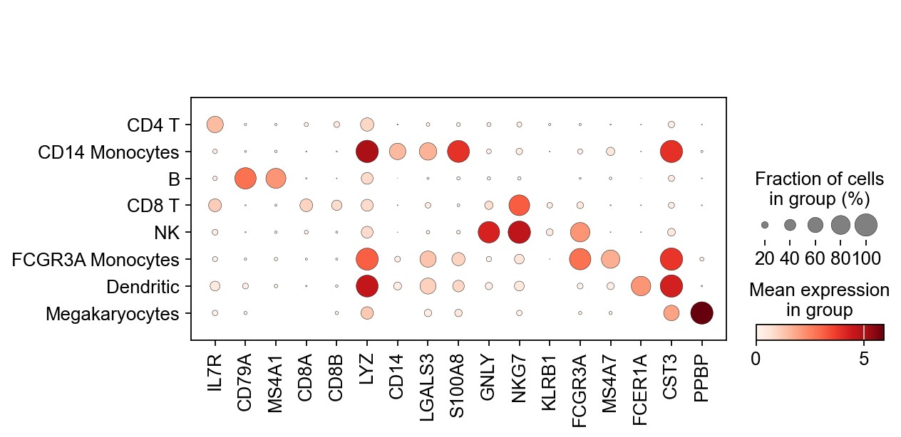
1 | # dotplot for marker genes |
e:\miniconda3\envs\pysc\lib\site-packages\scanpy\plotting\_dotplot.py:749: UserWarning: No data for colormapping provided via 'c'. Parameters 'cmap', 'norm' will be ignored
  dot_ax.scatter(x, y, **kwds)
1 | # violin plot |
1 | adata |
AnnData object with n_obs × n_vars = 2638 × 1838
    obs: 'n_genes', 'n_genes_by_counts', 'total_counts', 'total_counts_mt', 'pct_counts_mt', 'leiden'
    var: 'gene_ids', 'n_cells', 'mt', 'n_cells_by_counts', 'mean_counts', 'pct_dropout_by_counts', 'total_counts', 'highly_variable', 'means', 'dispersions', 'dispersions_norm', 'mean', 'std'
    uns: 'hvg', 'leiden', 'leiden_colors', 'log1p', 'neighbors', 'pca', 'rank_genes_groups', 'umap'
    obsm: 'X_pca', 'X_umap'
    varm: 'PCs'
    obsp: 'connectivities', 'distances'
总结
scanpy中scRNA-seq分析流程包括:
1 | # read in data |
由于后续需要在Geneformer中使用该数据,这里我将行名替换为ensembl id,并在细胞注释.obs中增加一列cell_type指定细胞类型和organ_major指定组织类型。同时,替换默认表达矩阵为原始counts。随后,以loom格式存储。
1 | # make dataset suitable for Geneformer |
| ensembl_id | n_cells | mt | n_cells_by_counts | mean_counts | pct_dropout_by_counts | total_counts | highly_variable | means | dispersions | dispersions_norm | mean | std | gene_name | |
|---|---|---|---|---|---|---|---|---|---|---|---|---|---|---|
| gene_ids | ||||||||||||||
| ENSG00000186827 | ENSG00000186827 | 155 | False | 155 | 0.077407 | 94.259259 | 209.0 | True | 0.277410 | 2.086050 | 0.665406 | -3.244448e-10 | 0.424481 | TNFRSF4 |
| ENSG00000127054 | ENSG00000127054 | 202 | False | 202 | 0.094815 | 92.518519 | 256.0 | True | 0.385194 | 4.506987 | 2.955005 | -1.157975e-10 | 0.460416 | CPSF3L |
| ENSG00000215915 | ENSG00000215915 | 9 | False | 9 | 0.009259 | 99.666667 | 25.0 | True | 0.038252 | 3.953486 | 4.352607 | 8.472988e-12 | 0.119465 | ATAD3C |
| ENSG00000162585 | ENSG00000162585 | 501 | False | 501 | 0.227778 | 81.444444 | 615.0 | True | 0.678283 | 2.713522 | 0.543183 | 3.502168e-10 | 0.685145 | C1orf86 |
| ENSG00000157916 | ENSG00000157916 | 608 | False | 608 | 0.298148 | 77.481481 | 805.0 | True | 0.814813 | 3.447533 | 1.582528 | 9.461503e-11 | 0.736050 | RER1 |
| ... | ... | ... | ... | ... | ... | ... | ... | ... | ... | ... | ... | ... | ... | ... |
| ENSG00000160223 | ENSG00000160223 | 34 | False | 34 | 0.016667 | 98.740741 | 45.0 | True | 0.082016 | 2.585818 | 1.652185 | 9.984445e-12 | 0.217672 | ICOSLG |
| ENSG00000184900 | ENSG00000184900 | 570 | False | 570 | 0.292963 | 78.888889 | 791.0 | True | 0.804815 | 4.046776 | 2.431045 | -3.911696e-10 | 0.723121 | SUMO3 |
| ENSG00000173638 | ENSG00000173638 | 31 | False | 31 | 0.018519 | 98.851852 | 50.0 | True | 0.058960 | 3.234231 | 2.932458 | -1.969986e-10 | 0.173017 | SLC19A1 |
| ENSG00000160307 | ENSG00000160307 | 94 | False | 94 | 0.076667 | 96.518519 | 207.0 | True | 0.286282 | 3.042992 | 1.078783 | 5.980517e-10 | 0.399946 | S100B |
| ENSG00000160310 | ENSG00000160310 | 588 | False | 588 | 0.275926 | 78.222222 | 745.0 | True | 0.816647 | 2.774169 | 0.629058 | -6.552444e-10 | 0.762753 | PRMT2 |
1838 rows × 14 columns
1 | # add cell_type and organ_major columns for cell |
| n_genes | n_genes_by_counts | n_counts | total_counts_mt | pct_counts_mt | leiden | cell_type | organ_major | |
|---|---|---|---|---|---|---|---|---|
| AAACATACAACCAC-1 | 781 | 779 | 2419.0 | 73.0 | 3.017776 | CD4 T | CD4 T | immune |
| AAACATTGAGCTAC-1 | 1352 | 1352 | 4903.0 | 186.0 | 3.793596 | B | B | immune |
| AAACATTGATCAGC-1 | 1131 | 1129 | 3147.0 | 28.0 | 0.889736 | CD4 T | CD4 T | immune |
| AAACCGTGCTTCCG-1 | 960 | 960 | 2639.0 | 46.0 | 1.743085 | FCGR3A Monocytes | FCGR3A Monocytes | immune |
| AAACCGTGTATGCG-1 | 522 | 521 | 980.0 | 12.0 | 1.224490 | NK | NK | immune |
| ... | ... | ... | ... | ... | ... | ... | ... | ... |
| TTTCGAACTCTCAT-1 | 1155 | 1153 | 3459.0 | 73.0 | 2.110436 | CD14 Monocytes | CD14 Monocytes | immune |
| TTTCTACTGAGGCA-1 | 1227 | 1224 | 3443.0 | 32.0 | 0.929422 | B | B | immune |
| TTTCTACTTCCTCG-1 | 622 | 622 | 1684.0 | 37.0 | 2.197150 | B | B | immune |
| TTTGCATGAGAGGC-1 | 454 | 452 | 1022.0 | 21.0 | 2.054795 | B | B | immune |
| TTTGCATGCCTCAC-1 | 724 | 723 | 1984.0 | 16.0 | 0.806452 | CD4 T | CD4 T | immune |
2638 rows × 8 columns
1 | # replace count matrix with raw counts |
array([[0., 1., 0.],
       [0., 0., 0.],
       [0., 0., 0.],
       [0., 0., 0.],
       [0., 0., 0.]], dtype=float32)
1 | # save in h5ad |
The loom file will lack these fields:
{'X_umap', 'PCs', 'X_pca'}
Use write_obsm_varm=True to export multi-dimensional annotations
e:\miniconda3\envs\pysc\lib\site-packages\loompy\bus_file.py:68: NumbaDeprecationWarning: [1mThe 'nopython' keyword argument was not supplied to the 'numba.jit' decorator. The implicit default value for this argument is currently False, but it will be changed to True in Numba 0.59.0. See https://numba.readthedocs.io/en/stable/reference/deprecation.html#deprecation-of-object-mode-fall-back-behaviour-when-using-jit for details.[0m
def twobit_to_dna(twobit: int, size: int) -> str:
e:\miniconda3\envs\pysc\lib\site-packages\loompy\bus_file.py:85: NumbaDeprecationWarning: [1mThe 'nopython' keyword argument was not supplied to the 'numba.jit' decorator. The implicit default value for this argument is currently False, but it will be changed to True in Numba 0.59.0. See https://numba.readthedocs.io/en/stable/reference/deprecation.html#deprecation-of-object-mode-fall-back-behaviour-when-using-jit for details.[0m
def dna_to_twobit(dna: str) -> int:
e:\miniconda3\envs\pysc\lib\site-packages\loompy\bus_file.py:102: NumbaDeprecationWarning: [1mThe 'nopython' keyword argument was not supplied to the 'numba.jit' decorator. The implicit default value for this argument is currently False, but it will be changed to True in Numba 0.59.0. See https://numba.readthedocs.io/en/stable/reference/deprecation.html#deprecation-of-object-mode-fall-back-behaviour-when-using-jit for details.[0m
def twobit_1hamming(twobit: int, size: int) -> List[int]:
Ref:
https://scanpy-tutorials.readthedocs.io/en/latest/pbmc3k.html#Clustering-3K-PBMCs